Lecture by Fields Medal winner Professor Dr Martin Hairer now online. He was the main speaker at the event organised by the German Mathematical Society (DMV), which was recently held at Bielefeld University.
Professor Dr Martin Hairer spoke on the topic of ‘Coin tosses, atoms, and forest fires’. Hairer is a leading expert in the field of stochastic analysis. Hairer teaches and researches at the École polytechnique fédérale de Lausanne and Imperial College London. He was awarded the Fields Medal in 2014 for his work on stochastic partial differential equations.
Thanks a lot for the very kind introduction and well, thank you very much for the invitation. It’s really a pleasure and honour to be giving this lecture. So since well, obviously the audience is quite mixed though, you know, professional mathematicians in the audience, but are also high school students in the audience. And so I thought I would start by asking a very simple question, which is what is actually mathematics? So you know, in school, a lot of what you do when you do mathematics in school, obviously, is you actually learn how to compute. I think the very beginning you learn how to multiply numbers, but then maybe you do a little bit more complicated computations, you learn how to solve equations or maybe how to differentiate functions or things like that. But I would say in a way, you know, computing is for mathematics, maybe a little bit like spelling or grammar is to writing. You know, obviously you need to know grammar in order to be able to write a book, but it’s not really the essential thing. And so if you want to be able to write a book, you need to actually come up with an original story of a very original plot. And that’s because you need to put it to paper, you need to write it. The important part of the story is the plot. It’s the story, but it’s not actually just the writing, even though, you know, of course, if you write well, you can use very beautiful language and that’s an important part of the book as well. It’s a bit similar with mathematics and computing. So actually, you know what’s what you see here on the slides are computers and so until the you know, the sixties or seventies beginning of computer was the job. I mean, now, of course, you have an electronic computers and even Finland, you have all of you have a very powerful computer with you in your pocket, which you call a phone. But it’s really a computer until the sixties. Computers, you know, being a computer was basically a job, but it was not a job for mathematicians either. It was sort of a medium skilled job, and you wanted to do it. If you could train for the job, it would be like a one month training or something like this. And then you could be a computer. So anybody can put out the computer pretty quick, then you can do it as a job. Well, now, of course, that Trump doesn’t exist anymore. But you could. And so so, you know, it’s mathematics isn’t computing. What is it? I mean, to some extent this we’re just exploring the world of ideas. And so it’s, you know, just like in the allegory of the cover of Plato, which I know probably most of you have seen that story, the idea being that, you know, we are a little bit like people who become here who only see shadows of the world of ideas out there. And you try to kind of make sense of this world of ideas was, you know, only this partial information that we see with these troubles that we still provoke, Wolf, to come. And in some sense, mathematics is really the exploration of this. This outside world is this world of ideas. And it’s you know, you try to some sense build confidence and see, you know, meaningful sentences about them, about objects that really have no logical contradictions. If you want to do that, you try to be as precise. You try to be absolutely precise in what you actually mean, right? A big problem often manages to be able to actually define things in a completely unambiguous way so that you really know what you’re talking about and so in that sense, being a mathematician is a little bit like the opposite of being a politician. So you know, he’s you’re a politician, then the imprecise is a feature because you want to you want to say something which means different things to different people, either because if you want to get elected, you want as many people as possible to kind of agree with you, but people don’t agree with each other. And so you have to say things which mean different things to different people. And then everybody can agree with you, even if they don’t agree with each other. So as mathematicians, you do precisely the opposite of that. Okay? So you try to be extremely precise so that when you say something, you know exactly what you’re saying and the person you’re talking to knows exactly what you’re saying. What. And so if you want, you know, all mathematicians in the world would always sort of agree on what the meaning of your sentence is. And so that’s basically the only way in which you can, you know, come up with really true statements. I mean, it’s a and nowadays, you know, is truth has sort of become almost like an old fashioned thing. I, I mean, if you look at what happens in politics nowadays, you know, basically people have become completely cynical and sort of nihilistic in a way and saying, well, actually, you know, you can just nevertheless think about truth and truth doesn’t exist anymore. So, I mean, mathematics is maybe kind of one of the rare places where you really have sort of absolute truth. But the really truth does little for as absolute as logic actually permits. And on. So that’s in some sense, you know, mathematics in general, this is very abstract provided. So you try to you build or you describe to school of logic. The concepts of mathematics has links to the real world. I mean, the reason why mathematics has been so successful is because of partly because of its applications to kind of describing the real world and the different ways in which it’s linked. So one way physics, I suppose the job of physicists in a way is basically to link mathematics to the real world, to come up with mathematical models that provide meaningful statements of, you know, real world phenomena, then of people doing modelling. So it’s sometimes physics and modelling, it’s almost the same thing, except that you can think of physics as going from the bottom up and modelling is going kind of pulled down in the sense that physicists try to have some kind of fundamental understanding of, you know, basic processes in the world. So you try to come up with very fundamental principles like conservation of financing, of conservation of mass or things like this. And then you sort of build the laws of physics on top of that, whereas if you do modelling, maybe you might be informed by the laws of physics, but if you would take more of a top down approach where you would say, well, maybe that phenomenon is sort of too complicated to actually figure out the laws that regulate itself from the bottom up. And so you try to just try to come up with some heuristics in order to kind of describe it. But still, you build a mathematical model in order to describe some phenomena of reality, and that doesn’t exist. So the way in which I think is which is somewhat special, which is how does the link between mathematics and computers in the way of computers, almost like the, you know, of a computer in the sense of, you know, your phone. It’s really like some sort of a physical embodiment of mathematics, I thought was what goes on in some sense inside of a phone. When you programme a phone, it’s essentially mathematics and it’s as close as you can get in some sense to a in the life manifestation of pure mathematics in the real world, in a way. Now personally I’m probabilistic, so my area of mathematics is probability theory. So most of this lecture is going to be about that. And so let’s stop. I mean, there’s one thing which is kind of interesting about probability theory, which is that, you know, we all have some sort of an intuitive idea of what the probability is. But, you know, people can still actually argue about it. If you think about it, it’s not completely clear. And maybe one reason for this confusion comes from the fact that to some extent there are really two different real world phenomena that we both call probability, and they are not quite the same thing. And the first one, if you want, is a subjective type of probability which is kind of related to your beliefs. So to be more precise, they don’t take the following situation, for example. So, you know, next year there’s going to be an election in the United States. And you can ask yourself whether Trump is going to be elected president. And I’ll take the statement, you know, please, what is the probability that he’s going to be elected now? So do you think the probability is, I don’t know, 40%? And what does this 40% actually mean? So that’s how I want to sell your piece of paper. Okay. And the piece of paper, if you own that piece of paper, then the day after the election, if Trump wins, you get €100. If he loses, you get nothing. And then the paper, the piece of paper is worthless. After that, the question is, how much are you willing to pay for that piece of paper? And the claim is that if you’re willing to pay, what’s the maximum amount you’re willing to pay on? So if you’re willing to pay 800, you know, like €99, that means that you’re really pretty certain that he’s going to win because otherwise you’re losing money. Well, if you only willing to pay €1 for it, you know, it basically means you’re not willing to buy it. And so it means you’re basically certain that he’s going to lose. And if you’re willing to pay €50, that means that you think he has a 50% chance of winning. If you’re willing to pay 70 you I mean, to show you a figure of a 70, he has a 70% chance of winning. That’s all. Okay. So that’s a kind of subjective if you want definition of probability and that’s for events that are kind of one off because that actually is going to happen one year from now. And I said it’s not going to be repeated tonight. It happens once. And that’s so there’s another type of probability that appears in situations where you have an experiment which is repeatable. So it’s an experiment where you don’t know, just like in the election, you don’t know the outcome, you can’t possibly predict the outcome. Like nobody has the information required to predict the outcome. Maybe even in principle it wouldn’t be predictable, but you can repeat the experiment and then you can ask yourself, you know, how often the different outcomes occur. And so that’s usually one the more sort of objective or a posteriori definition of a probability where you know, like for example, you roll the dice, you can roll the dice a thousand times. It’s the same experiment, even if it’s not exactly the same, in the sense that every time you roll it, you can roll in a tiny little bit differently. But but for all practical purposes, it’s the same experiment. It’s can repeat it as often as you want. And so they’re saying that the probability very come that you roll the six is one over six just means that, you know, if you roll it a million times about a sixth of the time, you’re going to get a six. I that’s if you want for the you know mathematicians in the audience in a way some of the difference between the evasion and the frequentist perspective which statisticians spend a lot of time arguing about. I mean, the claim is that it’s basically two different are just two different types of set ups and both of them arise in the real world. And it so happens that both of them are described by what we call probability theory, but actually just fundamentally slightly different things. But then once you have these probabilities of, you know, then we have various rules, what until we know that, for example, if you have different outcomes, so is the than the probability that one or the other happens is the sum of the probabilities. Is that mutually exclusive? Right. That’s the probability that you rule a six is one. Let’s take some of it into the one is also one of the six. The probability that you rule that one more thing one one over 349 and you multiply those in some sense and corresponds to multiplying is very independent, etc. So we have various rules of the work with these probabilities, but that’s just so important. You still have to assign them. Why do you have rules for working with these probabilities once you have them? For certain patterns? But you need to come up with these probabilities of of the simple events to start with. And there are essentially two guiding principles for doing the action. And the first one we’ve already seen in the examples for rolling off the die, which is symmetry. And so that’s the situation where you do an experiment. There are different outcomes and the different outcomes they are you are able to distinguish between them. But as far as the mechanism of the experiment is concerned, it doesn’t make any difference. And so this is like when you roll the dice, you can see whether it comes up one or two or three at a time. But if the die is completely symmetric, as far as the ruling is concerned, it doesn’t make any difference, you know, whether it’s in one position or in the other position. Same for passing the point. You can see whether it comes up and or tails. But as far as the coin is concerned, it doesn’t make any difference at all. And so in this case, well, if you’re in this situation like this where you have different outcomes of that, but you are able to distinguish. But the mechanism that produces that, you cannot distinguish between them, then it’s natural to assign equal probabilities for all of these outcomes. I’d like to rule that either ask it’s possible outcomes are completely indistinguishable, so each of them has probability one with six coin toss, each of them has a probability of a two. So there’s only two outcomes unless you’re really, really lucky. The contrast. And then there’s another principle which is more subtle, and that’s something which is much less intuitive, which is something called universality. And actually it’s quite fitting that, you know, Gauss’s name is attached to this actually for going to see this item. What is two part of this? So universality is this fact that actually in situations where, you know, you have some random outcome that is actually, you know, it arises from somehow many, many different kind of random events that combine in order to produce an outcome. Then very often in some kind of limited the probability distribution, distribution of the outcome doesn’t really depend very much on the details of the the probabilities that you assign to all of the random events that kind of combine to produce the outcome. So one, one way in which this arises is what’s called the Gaussian distribution, which is named for Gauss, the same policies, Gauss from the Gauss lectures. And so what’s the gas distribution? Well, for example, one thing you can do is you take imagine you take a coin and you toss it 100 times and you count how many times it comes up. And so if you toss a coin 100 times and you look at how many times it comes up head, well, on average it would come up 50 times. But, you know, typically it’s not exactly £50 either. I mean, sometimes it’s 27, sometimes it’s 51. But I don’t. And so maybe I took that experiment itself a thousand times and then I do a histogram. I look at, you know, how many times do I get 50? Has always I’m still against 51, 49 and so on. And so here I was done by the experiments I mean obviously and didn’t also coin 100,000 times. But I just ask the computer to do it and you know you get to is the wrong like this. So in this particular case you see for example fifties in the middle of the fifth, I actually got like 49 heads. So to be more often than I hundred and 51 against five people, often in 50. But it’s all of roughly distributed from some kind of curve like this. So if you do it 10,000 times or a hundred thousand times, I say it gets closer and closer to that curve. And that curve is called the distribution. And the beauty of it is that it’s the same curve. Controls are if you do that sort of statistics, you know, for pretty much any distribution. So here I, you know, just toss the coin and counted how many times it came up has included, for example, roll the dice and counted how many times I get the six, which is not quite the same thing I think is the probability of getting a six is only one of my six means of getting had is one or two. But you know, if you do the same kind of experiment, the curve that you’re going to get is going to be exactly the same. It’s going to be shifted a little bit on, you know, on selected small scale. The problem is going to be exactly the same curve. And in many, many situations, it’s basically always in a situation where you have like very small random quantities that are more or less independent and that you add up, you know, that if you produce a large quantity. So basically in every situation like that, this caption distribution shows up. And so then, you know, when you in a situation like this, you know that you get something off and you don’t actually really need to know the details of what’s the distributions of all the little things that add up to something big. Okay. And so that’s a really important principle because it tells us that we can basically make predictions on random systems, even if you don’t know all the details of the mechanism of how these systems work. Now, these two principles step, you know, the first principles seem pretty clear, right? I mean, the second principle is that’s my explanation is a bit of wishy washy. The first one seems very funny, but even the first one, you have to be a bit careful. So for example, think the following situation. So say I have two envelopes and the only information I give you so each of them has a checking and the only information I give you is that one of the checks has twice as much money as the other one. And then you open an envelope, you see what’s written on the check, you’re allowed to look at it. And then I give you a choice. So either you keep the money or you can change your mind. Okay? So you can take the other block if you want, which is either twice as much or half as much of this. If you change your mind, if you have all out to change boxes because you know, it’s the one with the smaller amount. And so the question is what should you do? Well, you know, if you change your mind, how much do you get the effort to save the first envelope you have asked yours? So then in the envelope, I lose, you know, half chance of this twice as much and half times does half as much. I told the average it’s a half times more powerful, but also half chances are twice as much, which is 5/4 of the value. So you should change your mind because again, on average you get five quarters of what you because if you don’t change your mind but it works for every value of x, fine. So you didn’t even need to know from the envelope to know that this. So you should have just chosen the other one before you even after that. I think it doesn’t make any sense. So so what’s the problem here? The problem is that, you know, it sounds like one of these situations doesn’t benefit, but they’re actually not. If you really think so, they replace the two by a thousand and so. So say the other option is the all the envelope, as I know a thousand times as much or on the 1000 times as off, you know, then it’s even clearer that you should change. I think it’s more it’s a half chance of getting thousand times more and a half chance of getting basically nothing. So you should always change because you get basically 500 times more. But now you know, let’s think sort of real world situation. You open the envelope, you see 10,000 in what you you’re actually going to do and you’re obviously not going to switch. And because I would be really crazy giving you that million you I don’t have to start this and so you know so you make it so the thing is you make it sounds like a cute little maths problem. They have this accent, it doesn’t mean anything, but there’s really a difference between €1,000 and €1,000,000. I So it’s actually not symmetric involved situation. And so, you know, this is sort of just a cute little problem. But you know, there is this is the trap one can fall into, which is to, you know, take some real world situation and turn it into a little cute little mathematical problem. And then, you know, you do the calculation, you get some outcome, and then you say, oh, yeah, okay. So this is, you know, what the outcome in the real world is supposed to be. And then you don’t realise that you’ve actually dramatically oversimplify what’s going on. And, and there are situations where this can have actually dramatic consequences. So there’s a case that happened, I don’t know, which was maybe ten, 15 years ago or something like that. In the U.K., there’s a lady called Sandy Clarke, and she has a child. And what it was I noticed a few months old sometimes, you know, babies actually die for unexplained reasons. Actually, it happens very rapidly. We find out it’s called Sudden Infant Death Syndrome and all that’s happened in that case. And two years later, she had another child and the same thing happened again. And so then some people got suspicious because this one, you know, what’s the chance that actually this will happen twice to the same family? So maybe she actually murdered her children. And so she was accused of murdering her children just on the basis that it would be extremely unlikely that this happens by itself. And so there was a trial and there was an expert witness who testified for the prosecution and said, well, you know, in a family of this and that social background, the probability of having sudden infant death syndrome for a child is about one in 20,000. And so the probability of having two children in the same family tying it all is one in 20,000 times more than 20,000. So it’s one in 400 million. And so it’s so unlikely, but this couldn’t possibly happen. And so she must have killed the tenant. I’m and she actually got convicted and she said, you know, seven or eight years in jail before the conviction was overturned. And, of course, it was overturned because, you know, the verdict was completely ridiculous. It’s down to the states, you know, so the first mistake is to think that one in 400 million is really small. I mean, one in 400 million is really small, but that’s 20 million families in the UK now, billions of families in the world. So the chance that it actually happens to some family is very high. I was just like, if you play the lottery, the chance that you win the lottery is very low. The chance that someone wins the lottery and you know, it happens every week. So I mean, here is, of course, the opposite of winning the lottery. But and the other mistake was to just multiply the probabilities because you can do that for independent things. But there’s no evidence that this is something independent. I think it may very well have some genetic component. As far as I know, it’s not completely clear. You know, if I mean, you can certainly imagine that there might be a genetic component to it. And then that means that if one child dies of sudden infant death syndrome, well, it may be because of some genetic reason. And if that’s the reason, there are good chances of the other child who has the same condition and would die for the same reason. But until you have one just naively multiplying the probabilities. So now let me come back to this other question. So this principle of beautiful solitude. And so I mentioned the Gaussian distribution, but I want to mention also maybe a more sophisticated type of universality that shows up, which is in some sense quite similar to discussing distribution. And so that’s related. That’s what’s called Brownian motion. And so Brownian motion, something was so it’s named after a problem problem. So he was a British botanist in the 1800s. And what he did is he he had a he was actually looking at pollen particles under a microscope. And so he had a sense of little pollen particles. And those microscope and what he was applied to here you see these particles and what you would see is actually something like this. And so you look at these particles under the microscope and you see them moving like this. I do make this a little jittery motion. And and so he was trying to understand why they do that. So, of course, it was very careful to kind of make sure that, you know, the water itself was not moving any more often. It wasn’t just because they were kind of being transported around. In the beginning, he thought, you know, maybe these are actually alive, but they are little like these tiny little animals that move around. But then he made sure to rule that out. We can make sure that, you know, there would be no like malnutrition for weeks or something and then beef off the weeks and was still doing the same. And so he it was pretty clear to him that they weren’t alive. And so so there’s this question of why. Why do you have this quantum motion? Where does this come from? And it’s actually a question. It’s interesting because those who live in Victorian England, well, this question did actually capture the imagination of the general public. So it was, you know, like a topic of conversation for high society. One was this question of, you know, can you actually understand the fly why there is this form, the emotion of this, the explanation that people came up with and sort of a quantitative version of this explanation was then actually provided by Einstein on the spot, which was good. So it’s the wall of ice and Feynman’s 1905 papers where, you know, it’s in two parts. So there’s the physical reason, of course, which we kind of all know now. And stocks, you know, water is made of molecules and the molecules of water, they really behave a little bit like little billion balls. So they’re kind of just moving straight lines. And if you want, the temperature of the water is kind of like the speed of these variables, all the animals in all directions and completely disordered in a good way. So now you’ll pull in particle. I mean, it’s a very small pollen particle, but it’s huge compared to a molecule of water. And so you have this huge pollen particle that gets bombarded by molecules of water from from all sides every time there’s a molecule of water that bounces off it, you know, it gives it a little push and push in one direction. But, you know, a molecule of water is so small that, you know, you basically don’t see the effect. But there’s billions and billions and billions of molecules of water that, you know, pushing it all the time. And the cumulative effect actually does make it move. And that’s what you see under the microscope on. And Einstein is philosophically they actually made time also quantitative in the way even to predict kind of by how much it’s supposed to move. And mathematically, the description they gave was in terms of what’s called the heat equation. So it’s basically saying, you know what, they did predict is how does the probability that the particle finds itself at a given location evolve over time? I think imagine you see the particle at some point and then you close your eyes and so it moves along randomly. And then you try to predict like 1 seconds later where it’s going to be since it moves randomly, you can’t tell for sure. The only thing you can give is sort of maybe some probability distribution. And it turns out that probability distribution is actually, again, the Gaussian distribution of the. On the other hand, it’s also related to the evolution of heat in the solid body. So imagine that you take instead of looking at how the probabilities evolve, you look at how heat evolved. So you take, for example, a piece of metal which is cold, and then you heat it up in one point and then you ask yourself, how does that hot spot kind of spread out? And that’s actually given mathematically, it’s given by exactly the same equation, which describes the evolution of probability. And so with that so since they have, you know, quantitative predictions, they have two ways of relating all the coefficients that drop in the equation to the microscopic description of water as being made of molecules that form it. It was so funny that these predictions and the reason why they were important is because at the time it wasn’t actually completely clear that matter is made of molecules and of atoms. And now, of course, we know that matter is made of atoms. And you can you can produce microscopes. Thisis really powerful physics. You see individual atoms a lot of the time it was sort of the prevailing hypothesis. So most people believe that mother is made of atoms, but there was a lot of competing hypotheses and there wasn’t really a single experiment that had no other explanation. And this was the first experiment that really had no other explanation. And the fact that water is made up of molecules and so so the fact that in half, two years later, he actually really experimentally verified it and, you know, he figured out that the predictions that Einstein was asking made for, you know, how far these particles move as a function of size and of this positive full time basis, if you will. That’s long. But this prediction was actually correct to within I know that like 10% around something that really kind of settled the debate about the existence of atoms and actually provided what the Nobel prise for that in 1926 precisely because it’s happened to be based on the existence of atoms. And what’s interesting is that about about the same time there was a young French guy for again and so he was interested in something completely different. So he was interested in what now we would call mathematical finance. And so he was interested in understanding the stock market and and so he wanted to understand how prices, you know, share prices evolve. And, you know, the story that he developed and his thesis was basically the following simple case that you have a share price and there’s lots of people buying and selling its shares. And every time somebody buys a sale, it creates a little bit more demand. So that actually drives the price up. And every time somebody sells, wants to sell a share, it kind of, you know, drives the price down. And I think many people would do that in most cases. You know, you and I was we sell shares for 100 or €4,000. It doesn’t have any effect on, you know, multibillion dollar companies. So the individual trades have tiny effects, most of them. But there’s many, many of them. And sometimes they drive the price up, sometimes they drive down. And so there’s a cumulative effect, which then makes the price move between us a little erratic and run away. And so you see, the story is basically exactly the same as the one with the wrong emotion, except that now the role of the grain of policy is played by, you know, the price of the big company and the role of the water molecules is paid by, you know, the investors buy the shares and sell the fast. And in his thesis, he also actually devised the heating collection. So he also set from air. So actually evolution of the plasma is described by this question and now this time it describes the probability that the price is rather than the probability of a position to certain values. And so that’s what’s basically, you know, the foundation of modern mathematical finance. And also, I think some of the more complex roles who then got the Nobel prise for not in economics but really didn’t really get much out of this. So he was in some sense he arrived too early somehow. And the you know, the French formulas of the time were not particularly impressed by his work. And they also, you know, thought it wasn’t terribly great, useful mathematics. And so how, you know, describes these lowly material questions of, you know, just prices of confidence and things like that. And so he had a really hard time actually finding a job. He had a job at the Sorbonne at this stage. But then there was World War One and he lost it. He had to go to fight. And when he came back, the trouble was gone. And then for most of his life, he was basically giving private lessons. And he, you know, he got his permanent job in his late fifties or something like that. So he was a bit unlucky. But then so you see the point of these two stories is that you have two situations that are in principle completely different. And on the one hand, you look at grains of pollen that move around in water. On the other hand, you look at the evolution of stock prices and then the stories that you tell about them are kind of similar. I think both cases there are sort of lots of little things that sort of cover the fact of the cumulative effect, sort of makes the last thing move around. That’s essentially the same stories in both cases. And by this universality, it somehow tells you that that’s actually the same mathematics long term behind both of these equations. And so if you want to actually make some real maths out of that, I tell you one. So, so I already mentioned that there’s some overheated question that is some real off but but that doesn’t really tell you how these things look like. What you would really want to do is, is to somehow say, well, you know, if I look at the trajectory of my stock price, for example, what does it actually look like? The function of time. So mathematically, what this means is that you want to construct something like a random a random continuous function, which tells you how the stock price moves. And that was actually done by Venus. So he was a mathematician, not M.A. in the finance. And so it looks like this one. Well, actually, I have a memory for that one. So here is the one. I am this horizontal one stock is vertical one. And so here you think there’s this idealised mathematical object which is now called the visa process, which describes this evolution, and that’s a random function. And here what I did is I taken one sample from that random function and then I kind of zoom it’s the same function and I just zoom out more and more. Honestly, it moves just because I’m zooming up. And this problem that you see is just to say that the way I’m doing now is the way that it’s the problem of face to face. Zoom out by a factor of two horizontally. I actually have to zoom out by square with this tool and the vertical. I’ve got to start the way of assuming that keeps the problem fixed for the next sitting across. If you want. And if you do that way of zooming out, then it always kind of looks the same. So it has some kind of fractal self, similar kind of behaviour. And then more recently what’s involved school for example. So here we proved the mathematical theorem in some sense quantifies the statement that, you know, many things that behave in that way. If you look at them on very large scales, they look like this being a process which is this idealised mathematical objects that I just showed you. Okay? And so now to to conclude, I wanted to give you a little bit of the mathematics that I’ve been talking about so far. It’s basic standard. In the fifties, it’s mostly 1820. This is this was 500 year old masterminds of. So what I want to do now is if you just a little glimpse into the bond model, like, you know, recent mathematics from the past five years, the last ten years. And so here the situation is. You ask yourself about fluctuations of interface growth models. Well, here’s the situation that you should imagine, is that there is a there’s a two dimensional surface, and it comes in sort of two types. For example, here at the surface is the forest, and there’s a forest fire. Okay? And so then there’s one half of the surface, which is the bit that was burnt. And then there’s the other part, which is the bit that’s not timber. And there’s an interface between the two which is the same form and the same from well here it clearly moves in one direction. It always moves in the not yet firm direction. And that what you see is you look at this flame formed and you see that it’s you know, it’s more or less like a straight line, but it’s not quite strength. And so it’s in the 14th arrondissement, you know, you know, this is because some bins burn a bit better, some bits are less well, but it’s the same bits where it was at the prospect that it was a bit slower. And so then you can ask yourself, you know, is there like some kind of idealised mathematical object that describes, you know, the fluctuations of the strange one? But now this time, it’s not just a random function of space. It’s a run on function of space and time because the function moves off like a random moving and the same situation shows up in different circles. And so here this is a picture from an experiment about liquid crystal. So it’s liquid crystal like the liquid crystal. So you have like you, a TV display and it’s a type of liquid crystal accounting in two phases. And they have different optical properties on the microscope. You see the difference. I suppose one type of looks, but the other one, the square and one is a bit more stable than the other one. So let’s say the the blackboard is a bit more stable than the grey one. And so what you do is you first preparing the grade state and then what you do is you take a laser beam and use little zap for laser beam across it. And when the unstable state got something off, I’m entering. It’s activated into the flips into the same state. So basically when you hit it with the laser beam, it turns black and then the black thing is more stable with actually the spot. And so what you actually see is first it’s a little break. The news happened with the laser beam, you see a black line and then the black line gets bigger because the black is more stable. And then the you know, the edge of the black line is what you see here. So it’s not quite straight. It seems to be a bit weakly like this. And then you ask yourself, how do these wiggles behave? Is that like a natural mathematical model for how they can also come up with just some, you know, random like mass models that have a similar feature? So for example here, this is what I call the Texas model to the Texas model is you just have Tetris bricks falling down on. And so here you just get the big pile of Tetris packs that you just imagine. The screen is like a Tetris game. So you have the Tetris bricks tumbling down, falling down the pylon, and you don’t plan on it. So they just tie it up until you see something like this. But and it’s a little bit similar, right, in the sense that now there are two regions that at the bottom is the region that sort of fill up with Tetris place. And at the top there’s the region which has no bricks yet. And while here there’s some sort of yeah, it’s sort of supposed to be roughly centred at the boundary between the two regions, but you don’t really see much, but you can zoom out. You see that we’ve had zoom out. Yeah, I see something like this. So now I’m running in my phosphor until the Tetris bricks kind of fall down super fast. And let me just pause this. All right, so now you really see I saw this. There’s the region here which is full of bricks. There’s the region here which has no bricks. And there’s a kind of interface here between the two which is, you know, vaguely like this. And the interface moves. Now it is moving it move. And now you can ask yourself, you know, if I zoom out more and more, do I get some kind of idealised thing, right? So I can I can zoom out even more, actually. I go even faster. You get something like this. So instead of like an idealised mathematical model, but this context, it’s just like there is this we have policies that describe some idealised form of emotional stock prices. So in this case, this is something called which has now been described. But this is my point from the last five or six years or something. So the first actual description of that object was done in 2016, I think of 15 or something like this was very expensive and recent and what can actually describe this object. But for example, the understanding is still by far not as good as what we have for wrong emotions. So in the sense that there are a few toy models, for example, for this Tetris bricks model, there is no theorem at all. I mean, sort of fairly simple feelings, but they basically say nothing about the fluctuations of. There are a couple of very, very specific mathematical models that are little bit similar to this Tetris big model for which one can actually show them, you know, if one zooms out in the correct way of smoothing out, that there is a limit and you can actually describe the limit. But the description of the limit is rather complicated. And it’s kind of interesting because the description of the limit relates to some of these different variables, plus the balance, which is called Run the Matrix Theory, which in prison has no business showing up. You know, and we saw this situation here about a thing which is much better understood me is situations where citations are symmetric. Also year fluctuations were completely asymmetric in the sense that you know, the Tetris bricks, the only pylons, they only go up, they never go down. The flame front always burns in one direction. You never retreat on them. And once the forest is burned, experiment’s not going to earth again. Save for the liquid crystal and it’s always the black one that in place the hydrogen region will never be able to Iraq. But there are other situations where you can imagine, you know, two regions competing and they compete on equal footing. And then, you know, the fluctuations can kind of go both ways. And those are much better understood. And then one actually understands very well what the limited movie is, if you want, and it has a description which is much more like some of Brownian motion in terms of cash and distributions, kind of. And so then what can ask oneself, you know, what if we’re in a situation where it’s not symmetric but almost symmetric, I will say there’s two regions. One of them is a tiny bit more stable than the other one. And so it’s kind of whatever it takes to invade the other region, but very slowly and for most of the fluctuations are quite symmetric. But then, you know, it invades a little bit and then it turns out that, well, if you zoom out by not too far, what you see is basically the same as if it was symmetric. It’s a zoom out by a lot, but what you see is exactly the same as if it was completely asymmetric. And there’s one you know, there’s what’s called the crossover regime where you somehow move from one situation to the other one. And it turns out that that also has some kind of universal behaviour. So there’s an equation that shows up which is complicated is the equation which I wrote down here, which is a stochastic partial differential equations, and it’s kind of a universal equation that describes the crossover regime. And so that by now, as you know, a number of theorists that have been involved in, you know, which really tell you that there are many situations of that type where that exact same equation actually shows up and describes this kind of crossover regime. And the interesting thing about that equation is that so I don’t want to go over it because this is a sample of the actual. But there is this term here which is the square of the slope of the solution. But you see already you’ve seen a little from the movie. These things tend to be really quite rough. I’ve I’ve actually seen you do a I have another movie here for the the solution of this equation kind of looks like this. And in fact, what you see here is that if I freeze this movie, I don’t know, $1 here falls on, so I’m not going to see the time. Okay. Anyway, you can kind of imagine what it looks like if it’s frozen, if you freeze this movie and you see that it kind of looks like one of these. But the emotions, you know, in space time and that we saw that it was self cinema was this sort of problem the motion might which means that basically at every point the slope is kind of incident and because it’s almost tangent to that problem comes it’s zooming up and it brings up, you know, that equation is just complete nonsense because this here is the square of the slope of the slope is infinite at every point. And so it’s part of the equation on the right hand side, that’s just the big infinity. And while this we with simple here are not spitballing, that’s the thing that makes it harmful and ultimately that makes it very irregular. And so in a way, you have to really write the equation right next to with a kind of minus and trinity and then what does that mean? So for we have the equation part and you know, so down on the part of the material I’m actually on the on right is you can ask yourself to do equations like that. Actually we have a V, right? And it’s not just like it’s not just about what kind of mathematical questions really. You know, they show up and show you the kind of models for the show up and then you can, you know, really compare, you know, if you give it a mathematical meaning, this stuff isn’t really the same as the thing that actually shows up on. And it turns out that you can do that. And I think I stop here. Thank you very much for your attention.
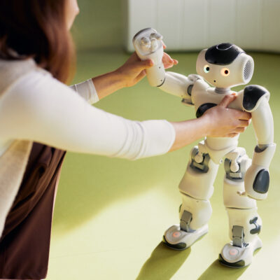
Dr Andreas Daniel Matt, Managing Director of IMAGINARY gGmbH, gave the accompanying lecture to the 40th Gauss Lecture. In his presentation, he talked about experiments with art, artificial intelligence, music and climate change.
It’s a great honour for me to be here today and I’m very happy to take you or, if I may, you on a journey together for the next 50 minutes. We have quite a lot planned, an interactive journey and to prepare for this there is a call to experiment or play along. This means that if you have laptops, iPads or tablets or mobile phones with you and want to, you are welcome to unpack them and I will explain how it works and you can play along. So we’re experimenting here and it’s also an overall experiment here with a full lecture theatre to carry out experiments, so this is a double experiment today. Exactly, this is the first travel preparation, the second travel preparation. Here, questions are more important than answers, I’ve added an asterisk here, answers are also important, but I think as a mathematician, asking questions is totally important and the joy of not understanding, that’s perhaps the first thing you have to learn when you study or do maths, that you’re really happy when you don’t understand something, because then you can learn something new again and somehow have a challenge again. I invite you to ask questions quietly now, perhaps we can also ask them out loud afterwards, but to ask the questions and explore the not-understanding here, you can ask lots and lots of questions. So, how does that work? You’ll find the link on the second page of the programme on the left and the QR code again. But you can also memorise t1p, you have to remember it by heart, .de is simple and cfg is Karl-Friedrich Gauss, so t1p.de slash Karl-Friedrich Gauss. To make things even easier, I always include the website in the top right-hand corner of all slides. Right, and we’ll start right away with the first experiment, a light billiard. If you have the website open, it looks like this. Here is the Gauss lecture and here are lots and lots of links. Let’s see how much we can manage. Sometimes there’s more information about the individual things here. We’ll start now with the first light billiard. So, how does a light billiard work? I have a beam of light that I send out. The circles we see here are mirrors and the beam of light goes in and comes out at the same angle. We do this again and again. We iterate the beam of light, so to speak, and we can make the circles bigger and smaller here. We can move them and we can also place the beam of light into the circle, for example, and then adjust the angle at which the beam of light is placed. We can make it bigger and smaller and can now experiment quite well. For example, you can simply disrupt a very symmetrical pattern by inserting a small circle here, for example, and get chaotic behaviour. It’s also really exciting. You have something beautifully symmetrical and you make a small change here, such a small disruption and it immediately becomes chaotic. They can ask themselves or you can ask yourselves what happens. Can I predict where this beam of light will end up after 100 iterations, for example, and you can also take a circle here, for example, and move it around and create beautiful patterns. There’s a mathematician, Sultan Palma, who thought to himself, I’ll take these circular mirrors, give them a nice pattern and try to create patterns with them. So I make a grid on these circular discs. He designed a programme, which is also linked here under the information. You have to install the programme and then you can simply send this beam of light through these mirror grids and see what comes out. So you have a beam of light and what’s really exciting is that you can, for example, there are different grid formations here and there is, among other things, a Goethe Faust Part 1. He has a symbol card, which unfortunately I couldn’t find quickly yesterday, but he has, so to speak, converted the pattern of these light reflections into letters and has written the beginning of Goethe Faust here. I’ve also picked it out again here. You are approaching wavering figures again, which once appeared in the cloudy view, is codified here and the exciting thing is, if you look in here now, you naturally need a very high level of accuracy to write something like this. So if I take a look here, for example, the position, the height of this beam of light here, has 1039 decimal places. I’m going to go to the decimal point 100 and change it here, turn the five into a 4, for example, and then you can see that the result is completely different. In other words, if I turn this around, you can see that it’s not that easy and you have to use a lot of maths to calculate very precisely, but theoretically you could codify the whole Goethe fist here. First experiment. It continues. Let’s do a fish school simulation. We go back to our list and now have a simple dynamic system with fish, these are agents here and each fish swims according to certain rules. You have controllers here and you can say, fish please swim fast or slow, fish swim with your neighbours and with zero neighbours, okay, not much happens, please swim with your five neighbours and also swim towards your neighbours. Let’s see what happens and every fish does exactly the same thing. So every single fish moves according to these rules. Now you can try to somehow create a large school of fish. You say, okay, we make lots of neighbours, I have a school of fish or fewer neighbours, then they swim around like this and the exciting thing is that every fish does exactly the same thing, acts according to the same rules, but overall a global schooling behaviour is created. You can also feed the fish by clicking on them with the mouse. Of course, this always works well and these are objects where the fish can’t swim through. What’s exciting here is just such systems, I don’t know if any of you know the Game of Life, which is a cellular automaton, but it’s very similar in principle. You have exactly the same rule at every point, so to speak. You work a bit with your neighbours, just like here. So I already know where my neighbours are and in principle I can map all the algorithms in the world using rules like this. Right, next. Exactly, the link list remains online, so you can continue playing later at your leisure. Surfer, that’s a programme, was also briefly mentioned, with the Imaginary, with which we grew up and that’s an algebraic, i.e. a ray tracer of algebraic surfaces in real time. What does that look like? Exactly, it’s easy to see. I have a formula down here, it’s a polynomial equation, so in three variables. I have an x, y and z and can somehow take 2, 3, 4, 5 to the power of plus and times. I’m not allowed to use any sine functions here, so nothing complicated, and I can change something at the bottom here and then I can immediately see the area in space, the real area in space, so the zeros of this equation are immediately mapped. This is a programme that generates super beautiful images that you can also rotate here. You can zoom in and out here with a slider, so you can imagine that these surfaces that you see are cut off with a sphere, so depending on the surface, they are compact, so you can somehow capture them all around or they go on infinitely. So this one here would go on, so here it’s cut off, so to speak, and there’s also something like an a here, that’s a parameter that you can adjust here, so you can also build in parameters here and that’s a huge playground, so you can also just start somehow. Let’s say x is 0, this is the y and z can be anything, i.e. I have the y and z planes and can then say x times x is just one point here, x times y I have two planes, x times y times z I would already have three planes. This means that if I multiply here, I can add an image, because that is always equal to 0, you have to think about that and I can also do something like a sphere, for example x² plus y² plus z² is equal to 1, a classic sphere with a radius of 1. I can now zoom up a bit, here I have a sphere. If I want to add something else, for example a Saturn, then I add a y here, then I have a plane. I can also intersect, that’s quite interesting, so not just adding, that’s a bit more complicated now, you have to think about it algebraically, so I could now say the first equation squared plus the second equation squared and then I have to subtract something small, I’ll make an a now, then I have exactly the intersection between the plane and the sphere here. I have to subtract something small because otherwise I can’t see it. If it’s only a wafer-thin surface, then this ray tracer can’t visualise the surface, which means I can make a ring here, for example, by making the a a little bigger. What’s exciting is that if I don’t do minus a, but plus a, nothing happens here, of course, then it’s gone. It’s quite interesting here, if you open up here, there are a few example equations, there are some really exciting things. There was one here, back then it was still a pupil, later a student, a student, who invented this equation here. When you look at it, you think to yourself, okay, what does it become and you can then copy it into the programme and see that this is the equation of the spoon. Very practical, really nice, you often need a spoon equation like that. Exactly, you can also try it, here’s the equation, you can also see that it’s a bit tricky. Let’s see if it works. I’ll put the spoon in here, that’s also an experiment. The spoon is there, but I think if you zoom out further, you can see that the spoon is in the middle, but then it goes on somehow and what is also exciting is that these visualisations are not always correct. There are wafer-thin lines or singularities that are also difficult to find and there are even more equations here. So there’s the equation of the heart, I’ll show that too, because it’s quite beautiful. You might have seen that already. Oh, you have to insert one more time. Exactly, the syntax has to be correct of course, otherwise it won’t work. Okay, but there’s definitely a half equation too, something’s happened. I’ll have to have a look, I’ve now had my switching back and forth, doesn’t work so well any more. I’ll have to adjust it once, sorry. What’s exciting about this surfer is that a lot happened back in 2008, the Year of Mathematics, when many, many people created algebraic surfaces and gave them funny names, and there were competitions and exhibitions in many countries where you could experience this mixture of formula and form in a beautiful, aesthetically pleasing way. Later on, we also had a very difficult, open problem: how do you get a 3D print from this surface, from this re-created surface, where I actually only know the pixels, for example. Here you can see a few more examples of surfaces, also from these competitions, and what’s exciting, also because the programme is openly licensed, it was, for example, converted here into a dish by a chef, a Michelin chef in Malaga. He turned it into five-star mathematical cuisine and it also ended up on a fashion collection in Slovenia. It’s nice when maths goes mainstream, here with the formula on the label of the dress. Right, now we’re moving on to music. The next programme is called ScaleLab, the laboratory of scales. Now I have to have a look, switch the sound volume here. I’ll switch to a simple sine wave here and just switch to waveform here. Can you hear that? Exactly. Imagine a piano that has no keys, but on which you can play all the frequencies here. It would be like this. Of course you can play beautiful melodies. But now it’s usually the case that you only want a finite number of keys. That’s also easier for the music. In other words, you have to think about which tone, which frequency can I play down here? You can see the blue lines here. I can’t take all of them, so I take out certain ones. And now the question is, how do I tune my piano? Which ones do I take? And how can I build scales? And which notes sound really good together when I play several at the same time? Now it’s interesting, you can choose different tunings here. I’ll take the Pythagorean tuning. So, I’ll go back and play these two together, for example. As you can see, I’m now on twice the wavelength, so to speak. They also sound quite good together. If I play a third or a fifth here, it also sounds quite good together. Pythagoras’ theory was that if the numbers are small, then the notes sound nice together. So 3 over 2, i.e. one and a half times the wavelength or one and a half times the frequency, then it sounds good. And if the numbers are higher, then it doesn’t sound quite so good together. There are other visualisation options. Of course, how something sounds is always a bit subjective. If I now show these waves, these two frequencies together on the x-axis and y-axis, then you can see a nice picture here, for example. If I take two proximity keys, then the image wobbles and you could say that if the images are a bit more stable, then it actually sounds better. If they wobble, then it doesn’t sound so good together. Helmholtz, a physicist, had tried to find a theory and developed a so-called dissonance curve, where he says that if I take two tones here and they are both relatively far down in the curve, then it sounds good when played together. If they are close to each other, then it doesn’t sound so good when played together. And with this programme you can now use these analysis tools, and you also have a synthesiser here, you can make your own instruments and can now also play with tunings. You can also say, for example, I take an Indian raga with a keynote and now I also have other types of notes. Here, for example. You need all the notes from time to time. Now I have a very special exhibit. Let’s see if it works here too. The pink trombone is not a trombone, it’s about the voice. We can open that up. This is a mathematical model of a person’s vocal tract. Imagine you cut through it like this or look into it like this and can now adjust the intensity and also the pitch that is generated here, in the glottis, and then shape the space in between, so to speak, by moving the tongue here. So the pitch here. And sometimes I also need the nose for this. And now we can try, for example, La, La, you have to make the mouth like this. And the interesting thing is that it works surprisingly well. There are also videos on the internet where people sing or talk with it. It’s a bit difficult. You need several fingers to do it. The exciting thing is that I’m going to show you a real-life video. This is an MRI scan of a baritone. The mathematical model works using cylindrical discs. There are 44 cylindrical discs of different sizes in the model. And the air flows through them. So it’s also a numerical model of a flow equation. And the end result is a beautiful voice or a voice. And the nose is important. There’s still a nose plus nose here, you can’t see it in the picture, but that’s another cylinder sequence that’s part of it. Well, since we’re already talking about flow equations, let’s go straight to a programme called Navier Stroke. It’s a play on words, so we’ll see why in a moment. And now let’s dive into the mathematics of climate change. This is also a real-time simulation that can be used to simulate liquids or fluids, including gases. There are also various parameters where you can set the dispersion or viscosity, various things. It is preset here. This is a nice programme if someone has a tablet or something like that with them, with lots of fingers at the same time. It’s quite meditative here, liquids. You can play with liquids without spilling anything. And that’s also a lot of maths, it also requires a good graphics card, otherwise it wouldn’t run so smoothly and quickly. And exactly, these Navier-Strokes equations are solved in real time. I have also listed them here and can give you a brief overview of how they work, i.e. differential equation systems. And the aim here is to calculate the acceleration of the air, which is influenced by various forces. So there’s the air pressure, something like how you know that the air moves from a high pressure area to a low pressure area. Then there is the Coriolis force of the earth, the earth rotates quite quickly. Here, of course, there is also something like gravity and these parameters, the viscosity in the interior. The exciting thing is that these equations are very universally applicable, so they can also be used for, I have a simulation here from a friend who does glacier research, so both glacier ice moves with these equations, but also honey. The equations are relatively complicated and you can quickly rack your brains as to how they work. But there are nice, fast, numerical solutions, including, as we have seen, on the graphics card. So, now we’ve heard about research, let’s enter the world of artificial intelligence, which is also my own field of research, and start with a programme, with a neural network, which means neural numbers. And now I have, I’ll start with another one, there are different versions, I’ll start with the full version here. You can first play with a trained neural network. So I can enter a number here by hand and then see what the neural network recognises. So I can recognise a number, I can do something here, and then you can see this here in the middle, I’m sure it’s a 4, the higher the bars, the more certain the network is, and you can watch what happens, so to speak, I can also do something, I’m sure it’s an 8, well, the 8 has lots of loops, it’s also quite exciting, for example if you make an X, then the network usually thinks it’s an 8, why a 1 comes out here is also exciting. And here there is always the first task, can you trick the network, here you can already see that it is actually not a 1, but a 7, but this is due to the fact that this network was trained with the American digits, where the 1 is simply a dash. Exactly, so here you have a neural network that has already been trained. The exciting thing now is what a network like this looks like and how I can train such a network. Here I have a network that hasn’t been trained at all, it starts somehow randomly, gives an output somehow randomly, the bars aren’t particularly high yet, that’s not certain, and I can now say here, please, I’m training you now, network, I always show you a picture, and then the solution, so I show you a picture of a 5 and tell you that’s a 5, a picture of a 6 and tell you that’s a 6. Many images here, let’s say 6,000 images, stop me for a moment, and the network tries, I’ll also show you how, to adjust various parameters in the centre so that the end result is what you want. And here you can already see that I have trained this now, this was also in real time, here with 7,000 images and it already works pretty well. And the exciting thing about this technology is that now I don’t have to know what an 8 looks like or what a 4 looks like, I can simply, I need training data, I have a technology, a neural network, and it can then recognise this training data correctly. I don’t have to programme any rules, I just need, in inverted commas, this training data and I can train it here. Exactly, there are also different architectures for experts, you can choose how the network looks internally. Let me briefly show you a mathematical insight into such a network, i.e. the input that you have, which we calculate down to 28 by 28 pixels, i.e. a little smaller than you can see. These are then, I think, 764 individual colour values. The colour values are always between 0 and 1, which is a bit small here, but you can already see that 1 is white, then there are a few shades of grey and 0 would be black. In other words, I end up with a list of these 764 numbers between 0 and 1. I then feed this list into a neural network. Let’s take a look at a video of what that looks like. So I’ve got the picture here at the front, which is 784, 784 numbers, exactly, between 0 and 1, just this one number. And these numbers are now multiplied by the so-called weights. So I have a number, multiply it by the weight, so here first pixel 0, is a black pixel, times 2, comes out 0. I now do this for this image here, exactly, multiply by all the weights and then add them up. In other words, at the end I have a sum here and that is my connection to this one hidden neuron here. I then add a number in the centre, there is a so-called bias, which I also add. And, very excitingly, there is a so-called activation function, which means I cut off all negative numbers. I only send positive numbers through, 0 or positive. I always do this for all numbers, i.e. I multiply again with the weights, add it up again, add a number, the bias, so to speak, which controls how strong this link is here and then an activation function at the front and then the bar comes out at the end. Yes, I have recognised the number or not. Yes, it’s a 1 or a 2. So here I have 10 numbers at the end and these are exactly my 10 digits that should come out. The exciting thing is how the training in the centre works. The training means exactly that I have to adjust these parameters, these weights, so that in the end I get exactly what I want. I have briefly summarised what we have now looked at graphically, so to speak, here again in mathematical notation. It’s also quite nice, you can summarise it using matrices and then have the activation in one place at the end, so to speak. It’s a bit of a battle with lots of indices, because you then have lots of hidden neurons, lots of hidden layers, but in the end you can work it out quite simply and have an activation function and the rest is just multiplication and addition. So now the question is, how does this training work? So I have these weights, but how do I adjust these weights? And that’s where we go to the next experiment. It’s called Gradient Descent and it’s a game. You can play it with two people, I can play it alone. The backstory is that a pirate hid a huge treasure in the Caribbean hundreds of years ago, at the deepest part of the ocean of course. And now we’re here a few hundred years later with a research boat trying to unearth this treasure. We can go left and right with the boat and can send a probe to the bottom at one point. You can already see here that I have 20 probes to choose from, and time is running out. I’m not going to stress myself now. And the probe then determines how deep it is at this point and what the ground is like at this point. So, I can now send a probe down somewhere. And now it’s all about finding out how I can find the deepest part of the ocean as quickly as possible. As you can probably already imagine, there’s a steep drop here, for example. Then I’ll try to get further down here. Oh, it’s even steeper down here. I’ll try to get even further down. I’ve just applied an algorithm, namely gradient descent, one of the most important algorithms in AI, where the aim is to gradually approach a minimum. The minimum would be, here the error is 0. You could say that this is an error function, this curve. If you play again, the shadow is hidden in a different place, just for your information. It can also be really difficult. You can think about what would be a really difficult floor. For example, if there are lots of waves. Or a very flat floor with only one small spot. That is of course super difficult. You can see what the ground looks like here. But flat is never that good. You don’t know where you’re going. And of course there are also local minima. This is a local minimum here, for example. That means there’s no shadow in this spot. I’ll have to see if I can get any lower at any point. Maybe over there. Yes, that looks quite good. There, exactly. Now you can imagine, I know now, sometimes maybe not at all, am I in a local minimum? Am I even reaching a global minimum? That’s not so easy. But I know that if I go down, I will definitely reach a minimum at some point. A local minimum. And that’s quite good. And what we have done here is to adjust the parameters in one direction, so to speak. That would now be a parameter of this network. I make it larger or smaller. And minimising the error means that the network does exactly what I want it to do. So it recognises the number 5, for example, and then I just adjust the parameters. I can always do that step by step. Adjust these parameters. Here is a parameter, i.e. a direction. In the really large networks, I have millions of parameters or thousands of parameters. Right, exactly. Maybe here’s another picture. This is the training data from this example, the new numbers. You can see here, it was trained with a straight line for the 1. The interesting thing about these technologies or this technology is that it nevertheless generalises in some way. This means that it learns with the one stroke, but somehow it recognises if there is a little tick at the top, for example for the German 1, it is still recognised. Or if not, here with the 4, for example, there are also different spellings of the 4. And that is also the strength of these neural networks, if you don’t train them too precisely, that they can also generalise in this way. Right, I’ll have a look at the clock, we’ve got 20 minutes left, so I’ll just do a few more experiments. I’ve added some bonus experiments down here just in case. Also for later or for fun. I’m going to go into my own research area here. Stochastic processes in AI, in machine learning. So-called reinforcement learning. Let’s start with a game. The game works like this, we have cards here. I have 10 moves and I can reveal any tile. Let me start. There are random numbers hidden there. And the aim is to get the highest possible total in 10 turns. I can also turn over the same card again. Now the question is, what do I do with my second turn? Should I open a new one here, plus 9, minus 25, or should I take the plus 9? Maybe we’ll open another one. I still have 6 moves left. Okay, I’ll stick with the plus 9. Now it’s really exciting to see. You can now run a simulation. Here’s a Monte Carlo method. I simply run it a million times or a hundred million times. And think about where I open a new card. And where do I take the highest tile so far? How often do you think I try to discover something new in 10 turns? And where do I use the best number so far? Now I have 4, 5. What do you think? 4 or 5 times? Maybe one more time. All right, I’ll stay here for now. I’ll show you the statistics here. If you just do the maths here, you can see, for example, that if I always stick with the first card or always use a different card, the total is the same. Almost the same here. And the best thing is if I turn up 4 times and then stick with the highest card. In this example. Of course, it depends a bit on how the random distribution is here. We have tried to build a slightly more complicated random generator. Sometimes there are only negative numbers or very high numbers. But in general, there is this problem of where do I keep trying out new things and where do I stick with the best so far? I know this personally when I go into an ice cream shop and there’s chocolate, my favourite ice cream. But then there might also be sheep’s cheese or mint. And then the question is, should I try sheep’s cheese and mint or should I stick with the chocolate, play it safe and eat three scoops of chocolate? Of course, it could be minus 25, but it could also be plus 200, because the mixture is very tasty. You may also know this from holiday destinations. I go back to the same place or try something new. And that’s an interesting concept. Discovering something new or reusing something already tried and tested. And there’s a machine learning method here called reinforcement learning or order-recognising learning, if you like. And it’s about how agents can learn, now as a technology, quite differently from a neural network, without prior knowledge. In other words, I have a robot here and it has different actions or an agent, which can also be a computer game. And it has different actions and it gets a reward. It learns through rewards. It’s also like for humans, if I reach onto a hot hob, that’s a negative reward, if you like, or a punishment. Then I won’t do it again. If I eat the chocolate ice cream here, it makes me happy and then I’ll try to eat it again. So you hide actions that are good for you and avoid actions that are not good for you. And it’s a bit like here. So here he gets these sweets, the reward is good. If he runs into a lava field like this, he won’t get a good reward. And if he gets to the end here, then he gets a huge reward. The interesting thing about this learning is that I only have to define these rewards and the robot then tries to learn for itself. I just let it run around here and it learns. And you can imagine it like this, it’s used in chess, for example. Here this Alpha or also with Go, AlphaGo or these chess programmes. The reward is that you win in the end, but the robot has to work out the individual moves, how to get to the end. In other words, it has to try out actions, experiment, explore. This brings us back to the dilemma of utilising knowledge or exploring. So here, for example, if I say only explore, then it just drives around randomly. And if I say only exploit, then it will only ever take the best route. This robot here has been learning for a while now. I can also speed it up a bit. At the beginning, sure, it’s a bit random. I’ll have to see if it manages to get to its destination at some point. Does he drive around a bit randomly again. And what he’s doing now, he’s building up a knowledge map in the background. I open it up. And basically it just looks at what the expected reward is when I’m standing at a field. For example, up here next to the exit, what is my expected reward? He gets plus 50 at the exit, which means that if I’m one space ahead, he loses one for every space he drives, i.e. minus one. That means he gets 49. If he’s still close, he gets 48. That means he already knows up there, that’s always the best way to get there. He still has to discover the rest. The numbers change every time he drives around here. I can make him learn a little faster. And exactly, it takes a bit of time. And he builds up a value map, as it’s called, with the expected long-term rewards. And these then define the best actions for the robot. At the moment, it’s doing a mixture like this. You can see this bar at the bottom between exploiting and exploring. It exploits a little and explores a little. And you could say, for example, I’m only doing exploration now. Then he just drives around more randomly. He can still continue to learn. Or I could say, please take the best route. And down here he may not yet know where the destination is, but up here he may have already learnt it. And now you know, for example, that if he starts here, he already has the best route and then always drives straight to the finish. You can also look at the map again now. He always goes where there are the highest rewards. And the great thing about this learning process is that it is very simple in algorithmic terms, i.e. in terms of computer science or programming. All you have to do is calculate from one field to the next and then from one field to the next. And in the end, he has also mathematically proven the best policy, in other words, the best way to reach the goal. And that is also very exciting here, that you can really prove that there is always such a best way in these processes. Well, let me see, maybe another example. What else can you do? Perhaps a logic game to finish off. Right, here we have an astronaut in space and she can only move if she encounters an obstacle. So here, for example, she could move downwards and would then stop in front of this satellite. And the aim is to get the astronaut to her rocket. So you can already imagine that here. And the same applies to the satellites. I can move them, but only until they land somewhere. So, for example, I can send the astronaut down here, then I can send the satellite over here, the astronaut over here and I’ve completed the first level. So, exactly, that’s still easy. Right, what are we doing here? Does anyone have a solution? I can’t see it right now. Could I send this one over there? Maybe up this way? Exactly, and on again. And it’s getting more and more difficult and what was the challenge here, there are many of these sliding puzzle games and here now for us, also as mathematicians, on the one hand to generate exactly the levels, i.e. to generate levels that are solvable. You can also do this iteratively or play through once, so to speak, and if I have a solution, then I have a level. But then, and this is the difficult part, defining the level of difficulty. When is a level difficult? And here we have a level generator, and every time you restart it, new levels are generated, but categorising when a level is difficult is not that easy and is also a big problem here in puzzle game mathematics. It’s not just the, so you can think about it, maybe the number of moves, but maybe sometimes it’s quite logical. I only have one move at a time and then the number of moves is not necessarily a clear indication of difficulty. Or, as we saw before, I might have to play the astronauts once in this direction, once in that direction or the satellites three times back and forth. And you can already see, so of course you could say, there is a lot more satellite interaction, for example, but this is a difficult level, for example, that doesn’t have that many satellites and you can think about how to play there. We work quite a lot with games in maths communication. Perhaps a little tip: the next International Mathematics Day, which is always on 14 March, has the motto Playing with Mathematics and there will also be lots of games. Well, I’m slowly coming to the end. There’s one more thing I wanted to say: Niki Kees is a person who does a lot of really exciting maths communication. I don’t know if anyone knows Niki. And Niki once said in a lecture that you should always show things first and only then talk about them. And since I heard that, I thought to myself, yes, that actually makes a lot of sense. That was also a bit of an idea here, you show the experiment and only then do you tell people what happens. And you often find yourself always wanting to tell first and show afterwards. That’s kind of ingrained in us. I explain what we’re doing, that’s how it works, that’s how it is, that’s how it is. But actually this moment, you’re already in the sandpit, you’ve already played and then there’s the physics of the sand and the water inside. Yes, it was mentioned before, very briefly, we develop these exhibits, very much software-based, but there are also a lot of physical things, always together with mathematicians. We are a non-profit organisation, so we come from the academic world, do everything non-profit, also worldwide, and have this openly licensed approach. This means that we develop an exhibit, it is often subsidised and then it can be copied worldwide. So many people, whether they are museums or universities, adopt these exhibits. And here is a tip for all future mathematicians or other scientists: we are working on a large project, also a DFG project, also together with the DMV, called MARDI, which is about mathematical research data infrastructure. And I’ve already mentioned that this open source logic is totally important here in science communication, but it’s even more important in research, so open science is the buzzword here. And an incredible amount is happening in the field of research data. And in mathematics, it is particularly difficult to see what all research data is. It’s just as much the formulae, the source code, models, of course also real data that you have, but basically everything you work with. And there are these so-called fair principles, which are about making this data fair. In other words, you store it in such a way that you can easily find it, that you can access it, so that there is no paywall or anything in between, or that the data also works together. So maybe I have a benchmark test here that also works with other data, that there are interfaces and that you can actually reuse the data. And this is a very large and very important project and I don’t think it can be mentioned often enough that we are trying to prepare the data in a sustainable way. Well, that brings me to the end and I’d like to thank you for this journey together and I’m happy to answer any questions.
Gauss Lectureship
The lecture series organised by the German Mathematical Society (DMV) is named after the famous mathematician Carl Friedrich Gauss, who lived in the 19th century and is widely regarded as one of the most important mathematicians of all time. The prestigious event honours his legacy and provides a platform for outstanding figures in mathematics to talk about current topics. Since 2001, the lecture has usually been held twice a year at different locations in Germany.